Revisiting Adaptive Multi-Arm Two-Stage Designs

ISBS, Madrid

Daniel Sabanés Bové (RPACT)

Silke Jörgens (University of Cologne)
Gernot Wassmer (RPACT)

October 15, 2026

Publications

Mehta and Kappler (2025)

Jörgens and Wassmer (2026)

Mehta and Kappler (2025)

• Compare the disjunctive power of stagewise and cumulative multi-arm multi-stage (MAMS) methods under different treatment selection rules and alternative hypothesis scenarios.
• They conjecture that non-consonance in closed testing plays a role in the greater power of the cumulative MAMS method over the stagewise MAMS method.
• Their conjecture that loss of consonance in the stagewise MAMS approach is responsible for the power loss has not been rigorously proven.
  • For consonant tests, rejection of the global intersection hypothesis implies rejection of at least one individual hypothesis.
• They propose a new R package AdaptiveGMCP for implementing the methods (which internally uses rpact for group sequential boundary calculations)

(Mehta and Kappler 2025, secs. 4–5)

Stagewise MAMS = Closed combination test

• The first approach is based on the inverse normal combination test:
  • Dunnett-adjusted $p$-values are calculated separately for both stages.
  • For each intersection test, the combination of stage 1 and stage 2 $p$-values is compared to the group sequential critical values derived by the chosen design.
• This procedure is commonly referred to as the closed combination test.

(Jörgens and Wassmer 2026; Bauer and Kieser 1999)

Cumulative MAMS = Adaptive Dunnett test

• The second approach uses the conditional error principle:
  • For each intersection hypothesis, the conditional error rate is calculated and the second-stage test statistic is compared to the corresponding critical value.
  • König et al. termed this the adaptive Dunnett test and proposed two variants that differ in whether the critical values are derived conditionally or unconditionally.
  • For the conditional version, in the case of known variance and without treatment arm selection, the adaptive and the classical (non-adaptive) Dunnett tests coincide.
  • Here we consider the conditional version of the adaptive Dunnett test.

(Jörgens and Wassmer 2026; König et al. 2008)

Treatment arm selection

• Both approaches allow for early stopping and treatment arm selection.
• In Mehta and Kappler’s investigation, sample size re-estimation is considered implicitly by fixing the total sample size for stage 2 and distributing it equally among selected arms.
• Treatment arm selection can be performed freely for both approaches.
  • There is neither a restriction on the number of treatment arms nor the requirement to select the arm that shows the highest treatment effect.

Previous power comparisons

• A power comparison between these approaches was previously performed already by Wassmer and Brannath.
• Their scenarios covered
  • three active treatment arms with a linear dose-response relationship
  • four selection strategies: select the best, select the two best, an $\epsilon$ selection rule, and no selection.
• They found that the fewer treatment arms selected, the smaller the power difference between the approaches was
  • If only one treatment arm is selected, the power difference was negligible.

(Wassmer and Brannath 2016, 2025)

Reasons for the power difference

• We do not agree with the conjecture that loss of consonance of the closed combination test is the main reason.
• Rather, there is a loss of power in the global test if $p$-values are computed by stage rather than overall
  • This means, in most cases where there is a rejection by the adaptive Dunnett test but not by the closed combination test, already the global test fails to reject.
  • This consonant failure of the closed combination test occurs in the majority of discordant test results.
• To show this, we performed a similar simulation study in which we specifically investigated the reason for failing each test by considering all intersection hypotheses.

Our simulation setup

• 10,000 simulation iterations per considered situation were performed with rpact (Wassmer and Pahlke 2025).
• Data were analysed with the closed combination and the adaptive Dunnett tests.
• The effect size scenarios are identical to those in the original paper by Mehta and Kappler (2025).
• We fixed the number of treatment arms to be selected, as the performance of the test procedures depends on how many treatment arms are selected rather than criteria for deselecting treatment arms.

(Jörgens and Wassmer 2026, Simulation Setup)

Effect size scenarios

Scenario	Arm 1	Arm 2	Arm 3	Arm 4
S1	0	0	0	0.25
S2	0	0	0.25	0.25
S3	0	0.25	0.25	0.25
S4	0.25	0.25	0.25	0.25
Emax1	0.069	0.125	0.200	0.250
Emax2	0.144	0.194	0.231	0.250

Selection options: all, best 3, best 2, best 1.

Comparison of disjunctive power per scenario

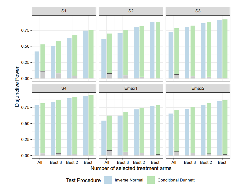
Disjunctive power: probability to reject at least one false null hypothesis. Blue and green: concordant cases; gray: consonant discordant cases; black: non-consonant discordant cases. (Jörgens and Wassmer 2026, fig. 1)

Results: overall small practical differences

• The power is somewhat higher for the adaptive Dunnett test compared to the closed combination test.
• However, uniformly across all scenarios, the difference between the power of the two tests is negligible if only the best treatment arm is selected.
• For most scenarios, this holds also true if the best two treatment arms are selected.
• A larger difference across all scenarios can only be observed if no selection takes place at all.
  • But in practice, an interim analysis for a study with four treatment arms would likely foresee some kind of treatment arm selection.

Results: discordant decisions

• The adaptive Dunnett test does not dominate the closed combination test in the sense that rejection in the closed combination test is always associated with rejection in the adaptive Dunnett test.
• Although the number of discordant results in this direction is much smaller, for all effect size scenarios and treatment selection rules there are constellations where there is rejection for the closed combination test but not for the adaptive Dunnett test
  • These are indicated by (very small) gray sections within the blue bars.

Results: non-consonance is a rare outcome

• Among the cases where the adaptive Dunnett test leads to rejection, but the closed combination test does not, the darkest segments represent the non-consonant discordant cases.
  • The global intersection test is rejected by the closed combination test, but none of the elementary hypotheses can be rejected.
• However, these cases are rare - in the vast majority of cases the origin of failure to reject lies in the global intersection test itself.

R example: designs setup

Now let’s have a look how easy it is to perform the simulations with rpact.

library(rpact)

# For closed combination test.
designIN <- getDesignInverseNormal(
  kMax = 2, alpha = 0.025,
  informationRates = c(0.5, 1),
  typeOfDesign = "noEarlyEfficacy"
)

# For adaptive Dunnett test.
designCD <- getDesignConditionalDunnett(
  alpha = 0.025, informationAtInterim = 0.5,
  secondStageConditioning = TRUE
)

R example: simulation function

simulate <- function(design, iterations = 10000L) {
  getSimulationMultiArmMeans(
    design = design,
    activeArms = 4,
    typeOfShape = "userDefined",
    effectMatrix = matrix(c(0.25, 0.25, 0.25, 0.25), nrow = 1),
    stDev = 1,
    intersectionTest = "Dunnett",
    typeOfSelection = "all",
    successCriterion = "atLeastOne",
    plannedSubjects = c(100, 200),
    allocationRatioPlanned = 1,
    maxNumberOfIterations = iterations,
    seed = 20261015
  )
}

# Obtain the power:
simulate(designIN)$rejectAtLeastOne

Note: plannedSubjects is cumulative per active arm, so here we have 100 (stage 1) + 100 (stage 2).

R example: S4 with all four arms retained

results <- lapply(
  list(
    "Closed combination" = designIN,
    "Adaptive Dunnett" = designCD
  ), 
  simulate
)
power <- sapply(results, function(x) x$rejectAtLeastOne[1])
knitr::kable(data.frame(
  Method = names(power),
  `Any-rejection estimate` = sprintf("%.1f%%", 100 * power),
  `Marginal MC standard error` = sprintf("%.1f pp", 100 * sqrt(power * (1-power) / 10000)),
  check.names = FALSE), align = c("l", "r", "r"))

Method	Any-rejection estimate	Marginal MC standard error
Closed combination	78.6%	0.4 pp
Adaptive Dunnett	82.2%	0.4 pp

R example: paired analyses

With this simple R function we can analyze each trial with both approaches, to obtain paired results for comparison.

analyze_trial <- function(dataSet, designIN, designCD) {
  stageIN <- getStageResults(designIN, dataInput = dataSet,
    intersectionTest = "Dunnett", normalApproximation = TRUE)
  stageCD <- getStageResults(designCD, dataInput = dataSet,
    intersectionTest = "Dunnett", normalApproximation = TRUE)

  IN <- getClosedCombinationTestResults(stageIN)
  CD <- getClosedConditionalDunnettTestResults(stageCD)
  
  # Identify the global intersection corresponding to all four active arms. Needed for the pairwise simulation function.
  global <- which(rowSums(IN$indices) == 4)
  stopifnot(length(global) == 1L)
  
  list(IN = IN, CD = CD, global = global)
}

dataSet: stage-specific means and sample sizes, standard deviations fixed to 1; control is the last group.

R example: discordant results

We wrote a simple function paired_simulation to generate paired trial results (available here).

It simulates each data set separately and applies the analysis function analyze_trial to obtain results for both the inverse normal (IN) and conditional Dunnett (CD) methods.

paired <- paired_simulation(
  nsim = 2000, keep = 4, effects = c(0.25, 0.25, 0.25, 0.25),
  seed = 20261015
)
trials <- paired$trials
cdOnly <- trials$CD & !trials$IN
inOnly <- trials$IN & !trials$CD

mean(trials$CD & trials$IN)          # colored left and right: both reject

[1] 0.778

mean(cdOnly & !trials$globalIN)      # gray on the right: IN global fails

[1] 0.0325

mean(cdOnly & trials$globalIN)       # black on the right: IN global passes

[1] 0.007

mean(inOnly & !trials$globalCD)      # gray on the left: CD global fails

[1] 0.0135

mean(inOnly & trials$globalCD)       # black on the left: CD global passes

[1] 0

R example: results

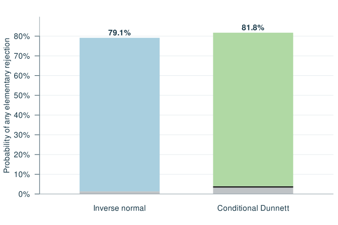
Blue / green: concordant cases.

Gray: consonant discordant cases; the global test for the respective other procedure is not rejected.

Black: non-consonant discordant cases; the global test for the respective other procedure is rejected, but no elementary hypothesis is rejected.

• IN gray segment: 1.35% (27 / 2,000).
• CD gray segment: 3.25% (65 / 2,000).
• CD black segment: 0.70% (14 / 2,000).

S4; all four arms; 2,000 iterations; no early efficacy. Simulation for this presentation, separate from the published results.

Comparison of the flexibility of the methods

• The inverse normal method can be easily extended to designs with more than two stages.
  • Although a recursive extension of the conditional Dunnett test is theoretically possible, the resulting calculations are likely to become quite complex.
• The adaptive Dunnett approach considered here is restricted to the case of known variance, an assumption that can be quite strong, particularly for small sample sizes.
  • In contrast, the inverse normal method naturally accommodates unknown variance by using Dunnett’s $t$ distribution if the residual variance estimate per stage is used.
  • In principle, one could also consider unknown variance, treating the variance as a nuisance parameter. This has been studied for the $t$-test, but was shown to be rather complex. (Gutjahr et al. 2011)

Conclusions

• The adaptive Dunnett approach has some power advantages over the inverse normal method with Dunnett’s test as intersection test for the closed testing procedure (closed combination test).
• However, in many relevant situations the power advantage is negligible.
• The closed combination test provides a more flexible framework, which can be used with more than two stages, with unknown variance, and of course also with other intersection tests beyond Dunnett’s test.
• Both tests are useful tools and can easily be used with the open source rpact package.

Thank you - Questions?

References

Bauer, P., and M. Kieser. 1999. “Combining Different Phases in the Development of Medical Treatments Within a Single Trial.” Statistics in Medicine 34: 1833–48.

Gutjahr, Georg, Werner Brannath, and Peter Bauer. 2011. “An Approach to the Conditional Error Rate Principle with Nuisance Parameters.” Biometrics 67 (3): 1039–46.

Jörgens, Silke, and Gernot Wassmer. 2026. “A Note on ‘A Comparison of Two Methods for Adaptive Multi-Arm Two-Stage Design’.” Statistics in Medicine 45 (6-7): e70448. https://doi.org/10.1002/sim.70448.

König, F, W Brannath, F Bretz, and M Posch. 2008. “Adaptive Dunnett Tests for Treatment Selection.” Statistics in Medicine 27 (10): 1612–25.

Mehta, C, and M Kappler. 2025. “A Comparison of Two Methods for Adaptive Multi-Arm Two-Stage Design.” Statistics in Medicine 44: e70162. https://doi.org/10.1002/sim.70162.

Wassmer, G, and W Brannath. 2016. Group Sequential and Confirmatory Adaptive Designs in Clinical Trials. Springer.

Wassmer, G, and W Brannath. 2025. Group Sequential and Confirmatory Adaptive Designs in Clinical Trials. 2nd ed. Springer.

Wassmer, G., and F. Pahlke. 2025. “rpact: Confirmatory Adaptive Clinical Trial Design and Analysis.” Https://Cran.r-Project.org/Package=rpact. R Package Version 4.2.